3.4 Gradients of a Vector Valued Functions

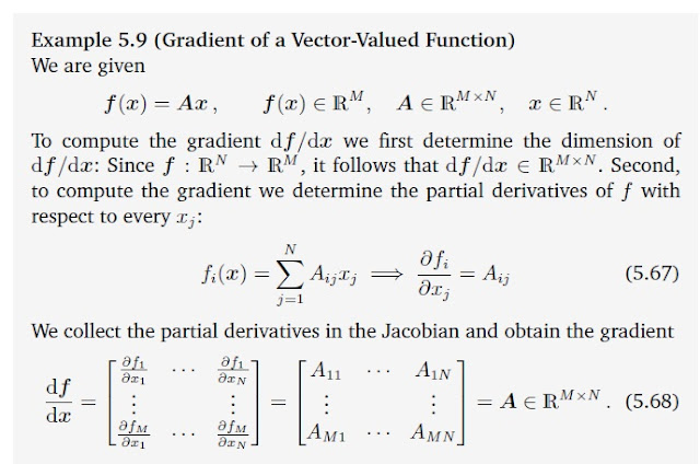
 We discussed partial derivatives and gradients of functions $f:\mathbb{R}^n \to \mathbb{R}$ mapping to the real numbers.Lets generalize this concept of the gradient to vector-valued functions(vector fields) $f: \mathbb{R}^n \to \mathbb{R}^m$, where $n \ge 1$ and $m \ge 1$.

For a function $f:\mathbb{R}^n \to \mathbb{R}^m$ and a vector $x=[x_1,\ldots,x_n]^T \in \mathbb{R}^n$, the corresponding vector of function values is given as

$f(x)=\begin{bmatrix}

f_1(x)\\

\vdots \\

f_m(x)

\end{bmatrix} \in \mathbb{R}^m$

where each $f_i: \mathbb{R}^n \to \mathbb{R}$ that map onto $\mathbb{R}$.

The partial derivative of a vector-valued function $f:\mathbb{R}^n \to \mathbb{R}^m$ with respect to $x_i \in \mathbb{R}$, $i=1,\ldots,n$, is given as the vector

We know that the gradient of  $f$ with respect to a vector is the row vector of partial derivatives, every partial derivative $\frac{\partial f}{\partial x}$ is a column vector. Therefore we obtain the gradient of $f:\mathbb{R}^n \to \mathbb{R}^m$ with respect to $x \in \mathbb{R}^n$ by collecting this partial derivatives

Definition: Jacobian

The collection of all first-order partial derivatives of a vector-valued function $f: \mathbb{R}^n \to \mathbb{R}^m$ is called the Jacobian. The Jacobian is an $m \times n$  matrix.

$J=\bigtriangledown _x f = \frac{\mathrm{d f(x)} }{\mathrm{d} x}=\begin{bmatrix}
\frac{\partial f(x))}{\partial x_1} & \cdots & \frac{\partial f(x))}{\partial x_n}
\end{bmatrix}$

As a special case of a function $f: \mathbb{R}^n \to \mathbb{R}^1$, which maps a vector $x \in \mathbb{R}^n$ onto a scalar, possesses a Jacobian that is a row vector of dimension $1 \times n $.

Remark: This is called numerator layout of the derivatives. i.e., the derivative $\frac{\mathrm{d f(x)} }{\mathrm{d} x}$ of $f \in \mathbb{R}^m$ with respect to $x \in \mathbb{R}^n$ is an $ m \times n$ matrix, where the elements of $f$ define the rows and the elements of $x$ defines the columns of the corresponding Jacobian. There exists also the denominator layout, which is the transpose of the numerator layout.

Lets consider an example with $x=\left [x_1 \quad x_2 \right]$.We define two vector valued functions $f_1(x)$ and $f_2(x)$.

If we organize both of their gradients into a single matrix, we move from vector calculus into matrix calculus. This matrix, and organization of the gradients of multiple functions with multiple variables, is known as the Jacobian matrix.

Example:

$f(x,y)=3x^2y$

$g(x,y)=2x+y^8$

Example Problems

1.Consider the following functions

A.$f_1(x)=sin(x_1)cos(x_2), x \in \mathbb{R}^2$

B.$f_2(x,y)=x^Ty,\quad x,y \in \mathbb{R}^n$

C.$f_3(x)=xx^T, \quad x \in \mathbb{R}^n$

a) What are the dimensions of $\frac{\partial  f_i}{\partial x}$

b) Compute the Jacobians.

A.

$f_1(x)=sin(x_1)cos(x_2), x \in \mathbb{R}^2$

$\frac{\partial  f_1}{\partial x_1}=cos(x_1)cos(x_2)$

$\frac{\partial  f_1}{\partial x_2}=-sin(x_1)sin(x_2)$

$J=\bigtriangledown _x f_1 =\begin{bmatrix}
\frac{\partial f(x)}{\partial x_1} & \frac{\partial f(x)}{\partial x_2}
\end{bmatrix}$

$J=\begin{bmatrix}
cos(x_1)cos(x_2)& -sin(x_1)sin(x_2)
\end{bmatrix}\quad \in \mathbb{R}^{1 \times 2}$

B.

$f_2(x,y)=x^Ty,\quad x,y \in \mathbb{R}^n$

$\frac{\partial  f_2}{\partial x}=\left[\frac{\partial  f_2}{\partial x_1}\quad \frac{\partial  f_2}{\partial x_2} \cdots \frac{\partial  f_2}{\partial x_n}\right]=\left[y_1 \quad y_2 \quad \cdots y_n \right]=y^T$

$\frac{\partial  f_2}{\partial y}=\left[\frac{\partial  f_2}{\partial y_1}\quad \frac{\partial  f_2}{\partial y_2} \cdots \frac{\partial  f_2}{\partial y_n}\right]=\left[x_1 \quad x_2 \quad \cdots x_n \right]=x^T$

$J=\begin{bmatrix}
\frac{\partial f(x)}{\partial x_1} & \frac{\partial f(x)}{\partial x_2}
\end{bmatrix}$

$J=\begin{bmatrix}
y ^T & x^T
\end{bmatrix}\quad \in \mathbb{R}^{1 \times 2n}$

C.

$f_3(x)=xx^T, \quad x \in \mathbb{R}^n$

2.Differentiate $f$ with respect to $t$ ( university question)

$f(t)=sin(log(t^Tt)) \quad t \in \mathbb{R}^D$

$f(t)=cos(log(t^Tt))\frac{1}{t^Tt}2t^T$

3.Compute the derivatives $\frac{\mathrm{d} f}{\mathrm{d} x}$ of the following functions by using the chain rule. Provide the dimensions of every single partial derivative. Describe your steps in detail.     ( university question)

$f(z)=log(1+z),\quad z=x^Tx\quad x \in \mathbb{R}^D$

4.Compute $\frac{df}{dx}$

$f(z) = sin(z) ; z = Ax + b ; A \in  R^{E\times D}; x \in R^D; b \in R^E$

where $sin(.)$ is applied to every element of $z$. ( university question)