Many algorithms in machine learning optimize an objective function with respect to a set of desired model parameters that control how well a model explains the data: Finding good parameters can be phrased as an optimization problem. Examples include: linear regression , where we look at curve-fitting problems and optimize linear weight parameters to maximize the likelihood.
A function $f$ is a quantity that relates two quantities to each other. These quantities are typically inputs $x \in \mathbb{R}^D$ and targets (function values) $f(x)$,which we assume are real-valued if not stated otherwise. Here $\mathbb{R}^D$ is the domain of $f$, and the function values $f(x)$ are the image/codomain of $f$.We often write
$f: \mathbb{R}^D \mapsto \mathbb{R}$
$x \mapsto f(x) $
to specify a function.
Example:
The dot product $f(x)=x^T.x , x \in \mathbb{R}^2$ would be specified as
$f : \mathbb{R}^2 \mapsto \mathbb{R}$
$ x \mapsto x_1^2+x_2^2$
Vector calculus is one of the fundamental mathematical tools we need in machine learning.We assume that the functions are differentiable.We will compute the gradients of functions to facilitate learning in machine learning models, since the gradient points in the direction of steepest ascent.
Differentiation of Univariate Functions
The difference quotient of a univariate function $y=f(x),x,y \in \mathbb{R}$ is
$\frac{\partial y}{\partial x}=\frac{f(x+\delta x)-f(x)}{\delta x}$
Computes the slope of the secant line through two points on the graph of $f$.In the figure these are the points with x-coordinates $x_0$ and $x_0+\delta x$.
The difference quotient can also be considered the average slope of $f$ between $x$ and $x + \delta x$.In the limit $\delta x \to 0$, we obtain the tangent of $f$ at $x$, if $f$ is differentiable.The tangent is then the derivative of $f$ at $x$.
The derivative of $f$ at $x$ is defined as the limit, for $h >0$
$\frac{\mathrm{d}f }{\mathrm{d} x}=\lim_{h\to 0} \frac{f(x+h)-f(x))}{h}$
and the secant in figure become tangent.
The derivative of $f$ points in the direction of the steepest ascent of $f$.
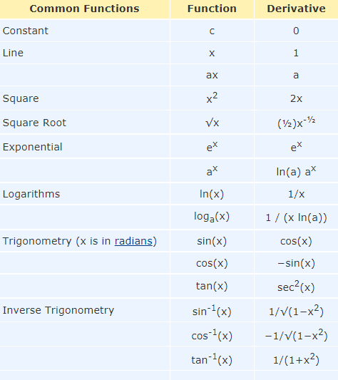
Example: Derivative of a polynomial $f(x)=x^n$
$\frac{\mathrm{d}f }{\mathrm{d} x}=\lim_{h \to 0} \frac{f(x+h)-f(x)}{h}$
$\quad=\lim_{h \to 0} \frac{(x+h)^n-x^n}{h}$
$\quad=\lim_{h \to 0} \frac{\sum_{i=0}^{n} \binom{n}{i}x^{n-i}h^i-x^n}{h}$
When $i=0$ $,\binom{n}{i}x^{n-i}h^i=x^n$.By starting the sum at 1, the $x^n$-term cancels and we obtain
$\frac{\mathrm{d}f }{\mathrm{d} x}=\lim_{h \to 0} \frac{\sum_{i=1}^{n} \binom{n}{i}x^{n-i}h^i}{h}$
$\quad=\lim_{h \to 0}\sum_{i=1}^{n} \binom{n}{i}x^{n-i}h^{i-1}$
$\quad=\lim_{h \to 0}\binom{n}{1}x^{n-1}+ \sum_{i=2}^{n} \binom{n}{i}x^{n-i}h^{i-1}$
The second term will $\to 0$ as $h \to 0$
$\quad=\frac{n!}{1!(n-1)!}x^{n-1}=nx^{n-1}$
Differentiation Rules
Product Rule: $(f(x)g(x))'=f '(x)g(x)+f(x) g'(x)$
Quotient Rule:$ \left(\frac{f(x)}{g(x)}\right)'=\frac{f '(x)g(x)-f(x)g'(x)}{g(x)^2}$
Sum Rule:$(f(x)+g(x))'= f ' (x) + g'(x)$
Chain Rule:$(g(f(x))'=g'(f(x))f ' (x)$
Chain rule is widely used in machine learning especially in neural network
Eg: lets compute the derivative of the function $h(x)=(2x+1)^4$, using the chain rule with
$h(x)=(2x+1)^4=g(f(x))$
$f(x)=2x+1$
$g(f)=f^4$
$f '(x)=2$
$g'(f)=4f^3=4(2x+1)^3$
So
$h'(x)=4(2x+1)^3. 2= 8(2x+1)^3$
Example Problems
1.Compute the derivative $f '(x)$ for $f(x) = log(x^4) sin(x^3) $$f '(x)=\frac{1}{x^4}.4x^3.sin(x^3)+log(x^4).cos(x^3).3x^2$
$f '(x)=\frac{4}{x}.sin(x^3)+3x^2.log(x^4).cos(x^3)$
2.Compute the derivative $f '(x)$ of the logistic sigmoid $f(x) =\frac{1}{1+exp(-x)}$
$f '(x) =\frac{1+exp(-x).0-1.-1.exp(-x)}{(1+exp(-x))^2}$
$f '(x)=\frac{exp(-x)}{(1+exp(-x))^2}$
where $\mu,\sigma \in \mathbb{R}$ are constants.
$f '(x)=f(x).-\frac{1}{2\sigma^2}2.(x-\mu)$
$f '(x)=f(x).-\frac{1}{\sigma^2}.(x-\mu)$
Learn More.....Examples


Comments
Post a Comment