1.9 Linear Mapping and Matrix Representation for Linear Mapping

Linear Mapping ( Linear Transformation)

A linear Mapping (or simply transformation, sometimes called linear transformation) is a mapping between two vector spaces: it takes a vector as input and transforms it into a new output vector. A function is said to be linear if the properties of additivity and scalar multiplication are preserved, that is, the same result is obtained if these operations are done before or after the transformation. Linear functions are synonymously called linear transformations.A mapping $\Phi:V \to W$ preserves the structure of the vector space if

$\Phi(x+y)=\Phi(x)+\Phi(y)$

$\Phi(\lambda x)=\lambda \Phi(x)$

for all $x,y \in V$ and $\lambda \in \mathbb{R}$

Definition:

For vector spaces $V$ and $W$, a mapping $\Phi: V \to W$ is called a linear mapping( or vector space homomorphism/linear transformation) if

$\forall x,y \in V \quad \forall \lambda, \psi \in \mathbb{R}:\Phi(\lambda x+ \psi y)=\lambda \Phi(x)+ \psi \Phi(x)$

Definition:Consider a mapping $\Phi: V \mapsto W$, where $V$ and $W$ are arbitary sets. Then $\Phi$ is called 

Injective (one to one) : if $\forall x,y \in V:\Phi(x)=\Phi(y) \implies x=y$

Surjective (onto): if $\Phi(V)=W$

Bijective(one to one and onto/injective and surjective)

If $\Phi$ is surjective, then every element in $W$ can be “reached” from $V$ using $\Phi$. A bijective $\Phi$ can be “undone”, i.e., there exists a mapping $\psi:W \to V$ so that $\Psi \Phi(x) = x$. This mapping is then called the inverse of $\Phi$ and normally denoted by $\Phi^{-1}$.

With these definitions, we introduce the following special cases of linear mappings between vector spaces $V $ and $W$:

Isomorphism: $\Phi : V \to W$ linear and bijective

Endomorphism: $V \to V$ linear

Automorphism: $\Phi: V \to V$ linear and bijective

We define $idv: V \to V, x \to x$ as the identity mapping or identity automorphism in $V$.

Theorem: Finite-dimensional vector spaces $V$ and $W$ are isomorphic if and only if $dim(V ) = dim(W).$

There exists a linear, bijective mapping between two vector spaces of the same dimension. Intuitively, this means that vector spaces of the same dimension are kind of the same thing, as they can be transformed into each other without incurring any loss.This also gives us the justification to treat $R^{m\times n}$ (the vector space of $m\times n$-matrices) and $R^{mn}$ (the vector space of vectors of length $mn$) the same, as their dimensions are $mn$, and there exists a linear, bijective mapping that transforms one into the other.

Remark: consider vector spaces $V, W,X$ Then

• For linear mappings $\Phi: V \mapsto W$ and $\Psi: W \to X$, the mapping $\Psi \circ \Phi:V \to X$ is also linear.
• If $\Phi: V \to W$ is an isomorphism, then $\Phi^{-1}: W \to V$ is an isomorphism too.
• If $\Phi:V \to W, \Psi: V \to W$ are linear, then $\Phi + \Psi$ and $\lambda \Phi \in \mathbb{R}$ are linear too.

Example:

Let $F: \mathbb{R}^2 \to \mathbb{R}^2 $ given by $F(x,y)=(xy,x)$, show that $F$ is not linear

We know that for linearity 

$F(\vec{v}+\vec{w})=F(\vec{v})+F(\vec{w})$

$F(c \vec{v})=c F(\vec{v})$

Let $\vec{v}=(2,3)$ and $\vec{w}=(3,4)$ and $\vec{v}+\vec{w}=(5,7)$

$F(\vec{v}+\vec{w})=F(5,7)=(5.7,5)=(35,5)$

$F(\vec{v})+F(\vec{w})=F(2,3)+F(3,4)=(6,2)+(12,3)=(18,5)$

It is noted that $F(\vec{v}+\vec{w}) \ne F(\vec{v})+F(\vec{w})$ So $F(x,y)=(xy,x)$ is not linear.

Matrix Representation of Linear Mapping

Let $\Phi(x):R^n \to R^m $ be a matrix transformation: $\Phi(x)=Ax$ for an $m \times n$ matrix $A$. 
$\Phi(u+v)=A(u+v)=Au+Av=\Phi(u)+\Phi(v)$

$\Phi(cu)=A(cu)=cAu=c \Phi(u)$

for all vectors $u,v$ in $R^n$ and all scalars $c$. Since a matrix transformation satisfies the two defining properties, it is a linear transformation.A linear transformation necessarily takes the zero vector to the zero vector.Most linear functions can probably be seen as linear transformations in the proper setting. Transformations in the change of basis formulas are linear, and most geometric operations, including rotations, reflections, and contractions/dilations, are linear transformations. Even more powerfully, linear algebra techniques could apply to certain very non-linear functions through either approximation by linear functions or reinterpretation as linear functions in unusual vector spaces.

Linear transformations are most commonly written in terms of matrix multiplication. A transformation$T: V \to W$ from $m$-dimensional vector space $V$ to $n$-dimensional vector space $W$ is given by an $n \times m$ matrix $M$. Note, however, that this requires choosing a basis for $V$ and a basis for $W$, while the linear transformation exists independent of basis.

The linear transformation from $\mathbb{R}^3 $ to $\mathbb{R}^2$ defined by $T(x,\,y,\,z) = (x - y,\, y - z)$ is given by the matrix

If $v = [x, \,y, \, z]$ Then the transformation is represented by the matrix vector product $M \times v$.

$T(v)=\displaystyle \left[\begin{matrix}1 & -1& 0\\0 & 1 & -1\end{matrix}\right] \displaystyle \left[\begin{matrix}x\\ y\\ z \end{matrix}\right]$

A common transformation in Euclidean geometry is rotation in a plane, about the origin. By considering Euclidean points as vectors in the vector space $\mathbb{R}^2$, rotations can be viewed in a linear algebraic sense. A rotation of $v$ counterclockwise by angle $\theta$ is given by

$\text{Rotate}(v) = \begin{pmatrix} \cos\theta & -\sin\theta \\ \sin\theta & \cos\theta \end{pmatrix} v.$$Rotate(v)=\displaystyle \left[\begin{matrix}cos\theta & -sin \theta\\sin \theta & cos\theta\end{matrix}\right]$

import numpy as np
import matplotlib.pyplot as plt
T=np.array([[2,0],[0,3]])
v1=np.array([1,2])
v2=T.dot(v1)
print("Red is the original vector-blue is the transformed vector")
plt.plot([0,v1[0]],[0,v1[1]],'r')
plt.plot([0,v2[0]],[0,v2[1]],'b')
plt.show()

o/p

Red is the original vector-blue is the transformed vector

Coordinate Transformation

consider a vector space $V$ and an ordered basis $B=(b_1,\ldots,b_n)$ of $V$. For any $x \in V$ we can obtain unique representation of $x$ with respect to $B$.

$x=\alpha_1 b_1+ \cdots + \alpha_n b_n$.

Then $\alpha_1,\ldots,\alpha_n$ are called coordinates of $x$ with respect to $B$, and the vector $\alpha=\displaystyle \left[\begin{matrix}\alpha_1\\ \vdots\\ \alpha_n \end{matrix}\right] \in \mathbb{R}^n$ is the coordinate vector/coordinate representation of $x$ with respect to the ordered basis $B$.

A basis effectively defines a coordinate system. We are familiar with the Cartesian coordinate system in two dimensions, which is spanned by the canonical basis vectors $e_1,e_2$. In this coordinate system, a vector $x \in R^2$ has a representation that tells us how to linearly combine $e_1$ and $e_2$ to obtain $x$. However, any basis of $R^2$ defines a valid coordinate system,and the same vector $x$ from before may have a different coordinate representation in the new $(b_1,b_2)$ basis.

Coordinate Transformation Matrix

Consider vector spaces $V$ and $W$ with corresponding ordered bases $B=(b_1,\ldots,b_n)$ and $C=(c_1,\ldots,c_m)$.Moreover we consider liner mapping $\Phi: V \to W$.For $j \in \{1,\ldots,n\}$.

$\Phi(b_j)=\alpha_1c_1+\cdots+\alpha_{mj}c_m=\sum_{i=1}^{m} \alpha_{ij}c_i$

is the unique representation of $\Phi(b_j)$ with respect to $C$. Then we call the $m \times n$ matrix $A_\phi$, whose elements are given by

$A_\phi(i,j)=\alpha_{ij}$

the transformation matrix of $\Phi$ (with respect to the ordered bases B of V transformation and C of W).

The coordinates of $\Phi(b_j)$ with respect to the ordered basis $C$ of $W$ are the j-th column of $A_\phi$. Consider (finite-dimensional) vector spaces $V,W$ with ordered bases $B,C$ and a linear mapping $\Phi : V \to W $ with transformation matrix $A_\phi$.

If $\hat{x}$ is the coordinate vector of $x \in V$, with respect to $B$ and $\hat{y}$ the coordinate vector of $y=\Phi(x) \in W$ with respect to C; then

$\hat{y}=A_\phi\hat{x}$

This means that the transformation matrix can be used to map coordinates with respect to an ordered basis in $V$ to coordinates with respect to an ordered basis in $W$.

Example:

Consider a homomorphism $\Phi: V \to W$ and ordered bases $B=(b_1,\ldots,b_n)$ of $V$ and $C=(c_1,\ldots,c_n)$ of $W$ with

$\Phi(b_1)=c_1-c_2+3c_3-c_4$

$\Phi(b_2)=2c_1+c_2+7c_3+2c_4$

$\Phi(b_3)=3c_2+c_3+4c_4$

The transformation matrix $A_\phi$ with respect to $B$ and $C$ satisfies $\Phi(b_k)=\sum_{i=1}^{4} \alpha_{ik}c_i$, for $k=1,\ldots,3$ and is given as

$A_\phi=[\alpha_1,\alpha_2,\alpha_3]= \displaystyle \left[\begin{matrix}1 & 2& 0\\-1 & 1 & 3 \\ 3 & 7 & 1 \\ -1 & 2 & 4 \end{matrix}\right]$

where the $\alpha_j, j=1,2,3$ are the coordinate vectors of $\Phi(b_j)$ with respect to $C$.

Example:

Lets consider a vector $[2,3]^T$ in standard coordinate system with bases $e_1=[1,0]^T$ and $e_2=[0,1]^T$

The coordinate of this vector in the new basis $b_1=[1,-1]^T$ and $b_2=[1,1]^T$ is

$\Phi(e1)=1/2 b_1+ 1/2 b_2$

$\Phi(e2)=-1/2 b_1+ 1/2 b_2$

So the transformation matrix is

$A_\phi=\displaystyle \left[\begin{matrix}1/2 & -1/2 \\1/2 & 1/2  \end{matrix}\right]$

The new coordinate vector is

$A_\phi . [2,3]^T=[-1/2,5/2]^T$

The Change of Basis Matrix

You can use a change of basis matrix to go from a basis to another. To find the matrix corresponding to new basis vectors, you can express these new basis vectors (i’ and j’) as coordinates in the old basis (i and j).

Using Linear Combinations

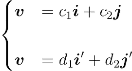
Let’s express the vector $v$ as a linear combination of the input and output basis vectors:

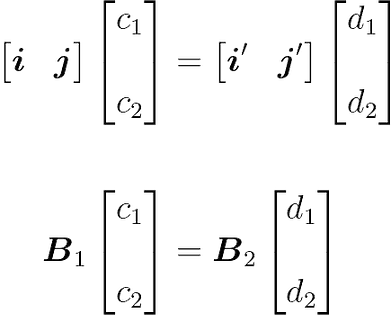
The scalars $c_1$ and $c_2$ are weighting the linear combination of the input basis vectors, and the scalars $d_1$ and $d_2$ are weighting the linear combination of the output basis vectors. You can merge the two equations:

Now, let’s write this equation in matrix form:

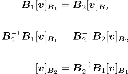
The vector containing the scalars $c_1$ and $c_2$ corresponds to $[v]B_1$ and the vector containing the scalars $d_1$ and $d_2$ corresponds to $[v]B_2$. We have:

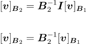
That’s good, this an equation with the term you want to find: $[v]B_2$. You can isolate it by multiplying each side by $B_2^{-1}:$

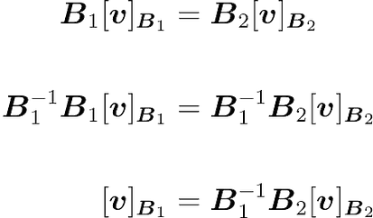
You have also:

The term $B_2^{-1} B_1$ is the inverse of $B_1^{-1} B_2$, which is the change of basis matrix $C$. This shows that $C^{-1}$ allows you to convert vectors from an input basis $B_1$ to an output basis $B_2$ and $C$ from $B_2$ to $B_1$.

In the context of this example, since $B_1$ is the standard basis, it simplifies to:

This means that, applying the matrix $B_2 ^{-1}$ to $[v]B_1$ allows you to change its basis to $B_2$.

Lets implement the previous example in python

Note that you have to consider the base vectors as column vectors of the matrix

import numpy as np

B1=np.array([[1,0],[0,1]])

B2=np.array([[1,1],[-1,1]])

c1=np.array([2,3])

print("Base B1- standard")

print(B1)

print("New Base B2")

print(B2)

print("coordinates in base B1")

print(c1)

print("new coordinate in new base B2")

c2=(np.linalg.inv(B2)).dot(B1.dot(v1.T))

print(c2)

print("converting back to the original base")

c1=(np.linalg.inv(B1)).dot(B2.dot(c2.T))

print(c1)

O/P
Base B1- standard 

[[1 0] 

 [0 1]]

 New Base B2

 [[ 1 1] 

 [-1 1]] 

coordinates in base B1

 [2 3]

 new coordinate in new base B2

 [-0.5 2.5] 

converting back to the original base 

[2. 3.]

Show that the mapping $T:(a,b) \to (a+2,b+3)$ of $V_2(R)$ into itself is not a linear transformation. Here $R$ is the field of real numbers. ( university qn)

Let $v_1=(a_1,b_1)$ and $v_2=(a_2,b_2)$

$T(v_1)=T(a_1,b_1)=(a_1+2,b_1+3)$

$T(v_2)=T(a_2,b_2)=(a_2+2,b_2+3)$

$T(v_1)+T(v_2)=(a_1+a_2+4,b_1+b_2+6)$

Similarly

$T(v_1+v_2)=(a_1+a_2,b_1+b_2)=(a_1+a_2+2,b_1,b_2+3)$

It is noted that

$T(v_1+v_2) != T(v_1)+T(v_2)$. So $T$ is not a linear transformation.