Row space, Column space and Null space

Row Space

The span of row vectors of any matrix, represented as a vector space is called row space of that matrix.

or

If we represent individual row as a vector, then the vector space formed by set of linear combination of all those vectors will be called row space of that matrix.

Assuming a 3x3 matrix $A=\begin{bmatrix}
1& 2 & 3 \\
4 &5& 6\\
7& 8& 9
\end{bmatrix}$


Then the row space is Span of these row vectors .
$Span( v1,v2,v3)$
where $v1=(1,2,3), v2=(4,5,6),v3=(7,8,9)$

If there are linearly depended vectors, we have to avoid those vectors.Linearly independent vectors can be found by converting the vectors into row reduced echelon form.For example consider

$A=\begin{bmatrix}
1& 2 & 3 \\
2 &4& 6\\
1& 1& 0
\end{bmatrix}$


After row reduction
$A=\begin{bmatrix}
1& 0 & -3 \\
0 &1& 3\\
0& 0& 0
\end{bmatrix}$


So the row space is the span of $[1,0,-3]$ and $[0,1,3]$.

Note: we can find transpose of $A$ and do the row reduction and get the pivot column which corresponds to the basis of the row space of the matrix.

Column Space

Similar to row space, column space is a vector space formed by set of linear combination of all column vectors of the matrix.

We can find the linearly independent vectors by row reduction and find the columns corresponds to the pivot column.

$A=\begin{bmatrix}
1& 2 & 3 \\
2 &4& 6\\
1& 1& 0
\end{bmatrix}$

After row reduction 

$A=\begin{bmatrix}
1& 0 & -3 \\
0 &1& 3\\
0& 0& 0
\end{bmatrix}$

The first and second columns are the pivot column.So the column space is the span of  $[1,2,1]$ and  $[2,4,1]$. the third column is a dependent column which is a linear combination of first two.

Both of these spaces have same dimension (same number of independent vectors) and that dimension is equal to rank of matrix.

Because, rank of matrix is maximum number of linearly independent vectors in rows or columns and dimension is maximum number of linearly independent vectors in a vector space (like column space or row space).

Rows and columns of a matrix have same rank so the have same dimension.

Null space

We are familiar with matrix representation of system of linear equations.

$Ax=0$

Here $A$ is coefficient matrix, $x$ is variable vector and 0 represents a vector of zeros.We can also find it’s solution (values of variables for which the equation above is satisfied) using Gaussian Elimination algorithm.

If we take a set of all possible solution vectors (all possible values of $x$), then the vector space formed out of that set will be called null space.

Or

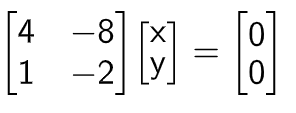
Null space contains all possible solutions of a given system of linear equations.Taking an example

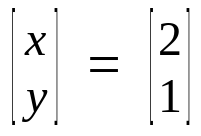
Solution vector of system of linear equations above is

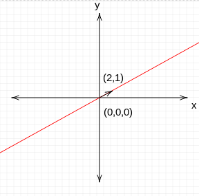
So this system of linear equations has two vectors in null space.[0,0] and [2,1].

Null space contains all the linear combinations of solution.Null space always contains zero vector.

Red line represents the null space of system of linear equations

Nullity

Dimension of null space is called nullity.
Nullity of the system above is 1.

Index theorem(Rank Nullity Theorem): For an $m \times n$  matrix  $A$,

$rank(A) + nullity(A) = n$

Null Space ( Python code)

from sympy import Matrix

M = Matrix([[1, 3, 0], [-2, -6, 0], [3, 9, 6]])

M.nullspace()

[Matrix([
[-3],
[ 1],
[ 0]])]

Finding nullity ( python code)

from sympy import Matrix

A = [[1, 2, 0], [2, 4, 0], [3, 6, 1]]

A = Matrix(A)

# Number of Columns

NoC = A.shape[1]

# Rank of A

rank = A.rank()

# Nullity of the Matrix

nullity = NoC - rank

print("Nullity : ", nullity)

Find a basis for the row space, column space and null space of the matrix given below ( university qn)

$A=\begin{bmatrix}
1& 3 & 0 \\
0 &0 & 1\\
0& 0& 0 \\
0 & 0 & 0
\end{bmatrix}$

The basis for the row space of $A$ is the two independent rows $(1,3,0)$ and $(0,0,1)$

The basis  for the column space of $A$ corresponds to the two pivot columns $(1,0,0,0)$ and $(0,1,0,0)$

The basis for the null space of $A$ is $(3,-1,0)$