Gradient Descent
Gradient Descent is a generic optimization algorithm capable of finding optimal solutions to a wide range of problems.
The general idea is to tweak parameters iteratively in order to minimize the cost function.
An important parameter of Gradient Descent (GD) is the size of the steps, determined by the learning rate hyperparameters.
If the learning rate is too small, then the algorithm will have to go through many iterations to converge, which will take a long time, and if it is too high we may jump the optimal value.
Note: When using Gradient Descent, we should ensure that all features have a similar scale (e.g. using Scikit-Learn’s StandardScaler class), or else it will take much longer to converge.
Types of Gradient Descent:
Typically, there are three types of Gradient Descent:
Batch Gradient Descent
Stochastic Gradient Descent
Mini-batch Gradient Descent
Stochastic Gradient Descent
Mini-batch Gradient Descent
Stochastic Gradient Descent (SGD):
The word ‘stochastic‘ means a system or process linked with a random probability. Hence, in Stochastic Gradient Descent, a few samples are selected randomly instead of the whole data set for each iteration. In Gradient Descent, there is a term called “batch” which denotes the total number of samples from a dataset that is used for calculating the gradient for each iteration. In typical Gradient Descent optimization, like Batch Gradient Descent, the batch is taken to be the whole dataset. Although using the whole dataset is really useful for getting to the minima in a less noisy and less random manner, the problem arises when our dataset gets big.
Suppose, you have a million samples in your dataset, so if you use a typical Gradient Descent optimization technique, you will have to use all of the one million samples for completing one iteration while performing the Gradient Descent, and it has to be done for every iteration until the minima are reached. Hence, it becomes computationally very expensive to perform.
This problem is solved by Stochastic Gradient Descent. In SGD, it uses only a single sample, i.e., a batch size of one, to perform each iteration. The sample is randomly shuffled and selected for performing the iteration.
SGD algorithm:

So, in SGD, we find out the gradient of the cost function of a single example at each iteration instead of the sum of the gradient of the cost function of all the examples.
In SGD, since only one sample from the dataset is chosen at random for each iteration, the path taken by the algorithm to reach the minima is usually noisier than your typical Gradient Descent algorithm. But that doesn’t matter all that much because the path taken by the algorithm does not matter, as long as we reach the minima and with a significantly shorter training time.
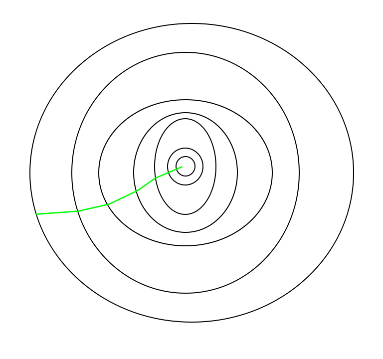
The path is taken by Batch Gradient Descent as shown below as follows:
A path has been taken by Stochastic Gradient Descent – 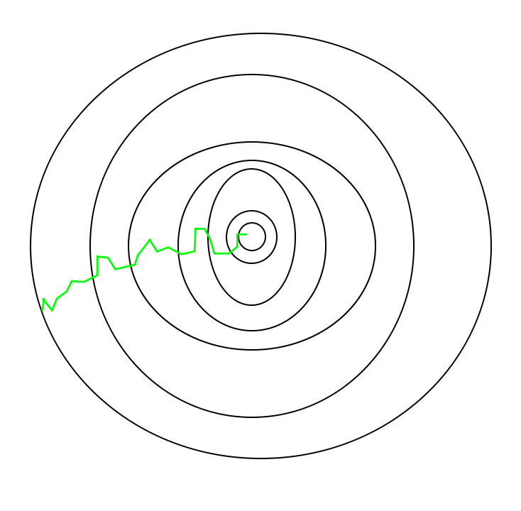
One thing to be noted is that, as SGD is generally noisier than typical Gradient Descent, it usually took a higher number of iterations to reach the minima, because of its randomness in its descent. Even though it requires a higher number of iterations to reach the minima than typical Gradient Descent, it is still computationally much less expensive than typical Gradient Descent. Hence, in most scenarios, SGD is preferred over Batch Gradient Descent for optimizing a learning algorithm.
| S.NO. | Batch Gradient Descent | Stochastic Gradient Descent |
|---|---|---|
| 1. | Computes gradient using the whole Training sample | Computes gradient using a single Training sample |
| 2. | Slow and computationally expensive algorithm | Faster and less computationally expensive than Batch GD |
| 3. | Not suggested for huge training samples. | Can be used for large training samples. |
| 4. | Deterministic in nature. | Stochastic in nature. |
| 5. | Gives optimal solution given sufficient time to converge. | Gives good solution but not optimal. |
| 6. | No random shuffling of points are required. | The data sample should be in a random order, and this is why we want to shuffle the training set for every epoch. |
| 7. | Can’t escape shallow local minima easily. | SGD can escape shallow local minima more easily. |
| 8. | Convergence is slow. | Reaches the convergence much faster. |
Comments
Post a Comment