1.10 Basis and Change of Basis

Basis

The basis is a coordinate system used to describe vector spaces (sets of vectors). 

To be considered as a basis, a set of vectors must:

Be linearly independent.
Span the space.

Every vector in the space is a unique combination of the basis vectors. The dimension of a space is defined to be the size of a basis set. For instance, there are two basis vectors in $\mathbb{R}^2$ (corresponding to the x and y-axis in the Cartesian plane), or three in $\mathbb{R}^3$.if the number of vectors in a set is larger than the dimensions of the space, they can’t be linearly independent. If a set contains fewer vectors than the number of dimensions, these vectors can’t span the whole space.

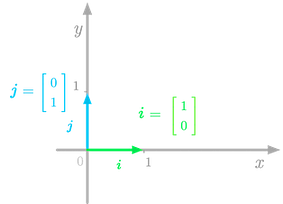
In the Cartesian plane, the basis vectors are orthogonal unit vectors (length of one), generally denoted as $i$ and $j$.

Figure 1: The basis vectors in the Cartesian plane.

For instance, in Figure 1, the basis vectors $i$ and $j$ point in the direction of the axis $x$ and $y$ respectively. These vectors give the standard basis. If you put these basis vectors into a matrix, you have the following identity matrix

$I_2=\displaystyle \left[\begin{matrix}1 & 0\\0 & 1\end{matrix}\right]$

Thus, the columns of $I_2$ span $\mathbb{R}^2$. In the same way, the columns of $I_3$ span $\mathbb{R}^3$ and so on.

Orthogonal basis

Basis vectors can be orthogonal because orthogonal vectors are independent. However, the converse is not necessarily true: non-orthogonal vectors can be linearly independent and thus form a basis (but not a standard basis).The orthogonal vectors are perpendicular to each other(90 degree apart) and their dot product is zero.

The basis of your vector space is very important because the values of the coordinates corresponding to the vectors depend on this basis. By the way, you can choose different basis vectors, like in the ones in Figure 2 for instance.

Figure 2. Another basis in a two-dimensional space. 

Keep in mind that vector coordinates depend on an implicit choice of basis vectors.

Coordinates and Linear combination

Any vector can be represented as linear combination of base vectors and are called the co-ordinates.

$\displaystyle \left[\begin{matrix}2 \\3\end{matrix}\right]= 2 \displaystyle \left[\begin{matrix}1 \\0\end{matrix}\right] +3 \displaystyle \left[\begin{matrix}0 \\1\end{matrix}\right] $ here the vector $[2,3]$ is represented as linear combination of base vectors $[1,0]$ and $[0,1]$ and the coordinate is $(2,3)$. suppose if the base vectors are $[1,-1] $ and $[1,1]$ then the coordinates become different

$\displaystyle \left[\begin{matrix}2 \\3\end{matrix}\right]= -1/2
\displaystyle \left[\begin{matrix}1 \\-1\end{matrix}\right]
+5/2
\displaystyle \left[\begin{matrix}1 \\1\end{matrix}\right]
$

Note that the coordinate become (-1/2 , 5/2).

Basis Change and new Transformation matrix

Lets look at how transformation matrices of a linear mapping $\Phi: V \to W $ change if we change the bases in $V$ and $W$. Consider two ordered bases

$B=(b_1,\ldots,b_n) \quad \tilde{B}=(\tilde{b_1},\ldots,\tilde{b_n})$ of  $V$

and two ordered bases of $W$

$C=(c_1,\ldots,c_m) \quad \tilde{B}=(\tilde{c_1},\ldots,\tilde{c_m})$ of  $V$

Moreover $A_\phi \in \mathbb{R}^{m \times n}$ is the transformation matrix of the linear

mapping $\Phi : V \to W$ with respect to the bases $B$ and $C$, and $\tilde{A_\phi} \in \mathbb{R}^{m \times n}$ is the corresponding transformation mapping with respect to $\tilde{B}$ and $\tilde{C}$.

Then $\tilde{A_\phi}$ is given as
$\tilde{A_\phi} = T^{-1}.A_\phi. S$

Here, $S \in \mathbb{R}^{n \times n}$ is the transformation matrix of  $idV$ that maps coordinates with respect to $\tilde{B}$ onto coordinates with respect to $B$, and $T \in  \mathbb{R}^{m \times m}$ is the transformation matrix of $idW$ that maps coordinates with respect to  $\tilde{C}$ onto coordinates with respect to $C$.

Definition(Equivalence):

Two matrices $A,\tilde{A} \in \mathbb{R}^{m \times n}$ are equivalent, if there exist regular matrices

$S \in \mathbb{R}^{n \times n}$ AND $T \in \mathbb{R}^{m \times m}$ such that $\tilde{A}=T^{-1}AS$.

Definition(Similarity):

Two matrices $A,\tilde{A} \in \mathbb{R}^{n \times n}$ are similar, if there exist a regular matrix

$S \in \mathbb{R}^{n \times n}$  such that $\tilde{A}=S^{-1}AS$.

 

Remark:Similar matrices are always equivalent. However, equivalent matrices are not necessarily similar.

Conclusion

Understanding the concept of basis is a nice way to approach matrix decomposition (also called matrix factorization), like eigen decomposition or singular value decomposition (SVD). In these terms, you can think of matrix decomposition as finding a basis where the matrix associated with a transformation has specific properties: the factorization is a change of basis matrix, the new transformation matrix, and finally the inverse of the change of basis matrix to come back into the initial basis .

Example and Python code