
Symmetric Positive Definite Matrix

 A real n\times n matrix A is symmetric positive definite if it is symmetric (A is equal to its transpose, A^T) and

x^T\!Ax > 0 \quad \mbox{for all nonzero vectors}~x.

By making particular choices of x in this definition we can derive the inequalities

\begin{alignedat}{2}     a_{ii} &>0                       \quad&&\mbox{for all}~i,\\     a_{ij} &< \sqrt{ a_{ii} a_{jj} } \quad&&\mbox{for all}~i\ne j.   \end{alignedat}

Satisfying these inequalities is not sufficient for positive definiteness. For example, the matrix

A = \begin{bmatrix}         1 & 3/4 & 0 \\         3/4 & 1 & 3/4 \\         0    & 3/4 & 1 \\        \end{bmatrix}

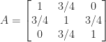
satisfies all the inequalities but x^T\!Ax < 0 for x = [1,{}-\!\sqrt{2},~1]^T.

A sufficient condition for a symmetric matrix to be positive definite is that it has positive diagonal elements and is diagonally dominant, that is, a_{ii} > \sum_{j \ne i} |a_{ij}| for all i.

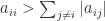
The definition requires the positivity of the quadratic form x^T\!Ax. Sometimes this condition can be confirmed from the definition of A. For example, if A = B^T\!B and B has linearly independent columns then x^T\!Ax = (Bx)^T Bx > 0 for x\ne 0. Generally, though, this condition is not easy to check.

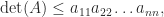
Two equivalent conditions to A being symmetric positive definite are

  • every leading principal minor \det(A_k), where the submatrix A_k = A(1\colon k, 1 \colon k) comprises the intersection of rows and columns 1 to k, is positive,
  • the eigenvalues of A are all positive.

The first condition implies, in particular, that \det(A) > 0, which also follows from the second condition since the determinant is the product of the eigenvalues.

Here are some other important properties of symmetric positive definite matrices.

  • A^{-1} is positive definite.
  • A has a unique symmetric positive definite square root X, where a square root is a matrix X such that X^2 = A.
  • A has a unique Cholesky factorization A = R^T\!R, where R is upper triangular with positive diagonal elements.

Sources of positive definite matrices include statistics, since nonsingular correlation matrices and covariance matrices are symmetric positive definite, and finite element and finite difference discretizations of differential equations.

Examples of symmetric positive definite matrices, of which we display only the 4\times 4 instances, are the Hilbert matrix

H_4 = \left[\begin{array}{@{\mskip 5mu}c*{3}{@{\mskip 15mu} c}@{\mskip 5mu}}             1 & \frac{1}{2} & \frac{1}{3}  & \frac{1}{4}  \\[6pt]            \frac{1}{2} & \frac{1}{3}   & \frac{1}{4}   & \frac{1}{5}\\[6pt]            \frac{1}{3} & \frac{1}{4}   &      \frac{1}{5}   & \frac{1}{6}\\[6pt]            \frac{1}{4} & \frac{1}{5}   &      \frac{1}{6}   & \frac{1}{7}\\[6pt]            \end{array}\right],

the Pascal matrix

P_4 = \left[\begin{array}{@{\mskip 5mu}c*{3}{@{\mskip 15mu} r}@{\mskip 5mu}}      1 &    1  &   1  &   1\\      1 &    2  &   3  &   4\\      1 &    3  &   6  &  10\\      1 &    4  &  10  &  20            \end{array}\right],

and minus the second difference matrix, which is the tridiagonal matrix

S_4 = \left[\begin{array}{@{\mskip 5mu}c*{3}{@{\mskip 15mu} r}@{\mskip 5mu}}      2 &   -1  &      &    \\     -1 &    2  &  -1  &    \\        &    -1 &   2  &  -1 \\        &       &  -1  &  2            \end{array}\right].

All three of these matrices have the property that a_{ij} is non-decreasing along the diagonals. However, if A is positive definite then so is P^TAP for any permutation matrix P, so any symmetric reordering of the row or columns is possible without changing the definiteness.

4\times 4 symmetric positive definite matrix that was often used as a test matrix in the early days of digital computing is the Wilson matrix

W =  \begin{bmatrix}        5 &7& 6& 5 \\        7 &10& 8& 7 \\        6& 8& 10& 9 \\        5& 7& 9 &10       \end{bmatrix}.

What is the best way to test numerically whether a symmetric matrix is positive definite? Computing the eigenvalues and checking their positivity is reliable, but slow. The fastest method is to attempt to compute a Cholesky factorization and declare the matrix positivite definite if the factorization succeeds. This is a reliable test even in floating-point arithmetic. If the matrix is not positive definite the factorization typically breaks down in the early stages so and gives a quick negative answer.

Symmetric block matrices

C = \begin{bmatrix}         A & X\\         X^T & B      \end{bmatrix}

often appear in applications. If A is nonsingular then we can write

\begin{bmatrix} A & X\\ X^T & B \end{bmatrix}  = \begin{bmatrix} I         & 0\\ X^TA^{-1} & I \end{bmatrix} \begin{bmatrix} A & 0\\ 0 & B-X^TA^{-1}X \end{bmatrix} \begin{bmatrix} I & A^{-1}X\\ 0 & I \end{bmatrix},

which shows that C is congruent to a block diagonal matrix, which is positive definite when its diagonal blocks are. It follows that C is positive definite if and only if both A and B - X^TA^{-1}X are positive definite. The matrix B - X^TA^{-1}X is called the Schur complement of A in C.

We mention two determinantal inequalities. If the block matrix C above is positive definite then \det(C) \le \det(A) \det(B) (Fischer’s inequality). Applying this inequality recursively gives Hadamard’s inequality for a symmetric positive definite A:

\det(A) \le a_{11}a_{22} \dots a_{nn},

with equality if and only if A is diagonal.

Finally, we note that if x^TAx \ge 0 for all x\ne0, so that the quadratic form is allowed to be zero, then the symmetric matrix A is called symmetric positive semidefinite. Some, but not all, of the properties above generalize in a natural way. An important difference is that semidefinitness is equivalent to all principal minors, of which there are 2^{n-1}, being nonnegative; it is not enough to check the n leading principal minors. Consider, as an example, the matrix

\begin{bmatrix}         1 & 1 & 1\\         1 & 1 & 1\\         1 & 1 & 0      \end{bmatrix},

which has leading principal minors 10, and 0 and a negative eigenvalue.

A complex n\times n matrix A is Hermitian positive definite if it is Hermitian (A is equal to its conjugate transpose, A^*) and x^*Ax > 0 for all nonzero vectors x. Everything we have said above generalizes to the complex case.


import numpy as np
A=np.array([[1,1,2],[2,2,3],[1,3,1]])
B=A.dot(A.T)
print("Symmetric positive definite Matrix B")
print(B)
x=np.array([1,2,3])
print("x.T A x >0")
print(x.T.dot(B.dot(x)))
eigva,eigv=np.linalg.eig(B)
print("eigen values")
print(eigva)
print("eigen vectors")
print(eigv)

o/p
Symmetric positive definite Matrix B
[[ 6 10  6]
 [10 17 11]
 [ 6 11 11]]
x.T A x >0
381
eigen values
[30.82496889  0.04141054  3.13362056]
eigen vectors
[[-0.42376703 -0.82534407 -0.37313358]
 [-0.73151695  0.55478298 -0.39635691]
 [-0.53413898 -0.10499055  0.83885191]]

Comments

Popular posts from this blog

Mathematics for Machine Learning- CST 284 - KTU Minor Notes - Dr Binu V P

  Introduction About Me Syllabus Course Outcomes and Model Question Paper University Question Papers and Evaluation Scheme -Mathematics for Machine learning CST 284 KTU Overview of Machine Learning What is Machine Learning (video) Learn the Seven Steps in Machine Learning (video) Linear Algebra in Machine Learning Module I- Linear Algebra 1.Geometry of Linear Equations (video-Gilbert Strang) 2.Elimination with Matrices (video-Gilbert Strang) 3.Solving System of equations using Gauss Elimination Method 4.Row Echelon form and Reduced Row Echelon Form -Python Code 5.Solving system of equations Python code 6. Practice problems Gauss Elimination ( contact) 7.Finding Inverse using Gauss Jordan Elimination  (video) 8.Finding Inverse using Gauss Jordan Elimination-Python code Vectors in Machine Learning- Basics 9.Vector spaces and sub spaces 10.Linear Independence 11.Linear Independence, Basis and Dimension (video) 12.Generating set basis and span 13.Rank of a Matrix 14.Linear Mapping...

Vectors in Machine Learning

As data scientists we work with data in various formats such as text images and numerical values We often use vectors to represent data in a structured and efficient manner especially in machine learning applications In this blog post we will explore what vectors are in terms of machine learning their significance and how they are used What is a Vector? In mathematics, a vector is a mathematical object that has both magnitude and direction. In machine learning, a vector is a mathematical representation of a set of numerical values. Vectors are usually represented as arrays or lists of numbers, and each number in the list represents a specific feature or attribute of the data. For example, suppose we have a dataset of houses, and we want to predict their prices based on their features such as the number of bedrooms, the size of the house, and the location. We can represent each house as a vector, where each element of the vector represents a specific feature of the house, such as the nu...

2.14 Singular Value Decomposition

The Singular Value Decomposition ( SVD) of a matrix is a central matrix decomposition method in linear algebra.It can be applied to all matrices,not only to square matrices and it always exists.It has been referred to as the 'fundamental theorem of linear algebra'( strang 1993). SVD Theorem: Let $A^{m \times n}$ be a rectangular matrix of rank $r \in [0,min(m,n)]$. The SVD of A is a decomposition of the form. $A= U \Sigma V^T $ with an orthogonal matrix $U \in \mathbb{R}^{m \times m}$ with column vectors $u_i, i=1,\ldots,m$ and an orthogonal matrix $V \in \mathbb{R}^{n \times n}$ with column vectors $v_j, j=1,\ldots,n$.Moreover, $\Sigma$ is an $m \times n$ matrix with $\sum_{ii} = \sigma \ge 0$ and $\sigma_{ij}=0, i \ne j$. The diagonal entries $\Sigma_i=1,\ldots,r$ of $\sigma$ are called singular values . $u_i$ are called left singular vectors , and $v_j$ are called right singular vectors .By convention singular values are ordered ie; $\sigma_1 \ge \sigma_2 \ldots \sigma_r \...